| Column | Description |
|---|---|
| experimentID | Unique identifier of the experiment. |
| trapID | Unique identifier of the trap used. |
| lineageID | Unique integer of the stem cell and its ancestry. |
| cellID | Unique identification number for each cell existing since the beginning of the experiment or generated later. |
| motherID | Unique identification number for each cell existing since the beginning of the experiment or generated later. |
| trackID | Indicates the x-y coordinates where the cell being tracked starts. |
| roiID | Indicates the x-y position in which the cell is located, followed after each photograph. |
| frame | Number of the photograph in the sequence of photographs taken, indicating the elapsed time (10 minutes per frame). |
| length | Cell length. |
| division | Indicates cell division events, represented by the value 1 when they occur and 0 otherwise. |
| GFP | Represents the relative fluorescence intensity in each cell by green fluorescent protein (i.e., GFP). |
| DsRed | Represents the relative fluorescence intensity for cells generated by rhodamine’s internalization (i.e., DsRed); an indicator of cell death events. |
| tracking_score | Determine how good or bad the tracking of a cell was. |
| state | Indicates the state of the cell determined from its length and fluorescence thresholds. -1 for death, 0 for normal, and 1 for filamentation (see Section 2.2 for detailed information). |
1 Image processing
1.1 Introduction
With the progress of technology, optical and fluorescence microscopy has become a fundamental tool for the characterization and understanding of the bacterial world. Microscopy has allowed humanity to extend its senses to observe the unknown world with exciting new perspectives they might never have envisioned otherwise. Furthermore, microscopy offers a clear advantage over other techniques that characterize bacteria since it can acquire data from living cells in spatial resolution (Schermelleh et al. 2019). (Schermelleh et al. 2019).
Microfluidic research techniques’ mechanical and intellectual development provides an excellent opportunity to overcome bio-medical and chemical techniques (Convery and Gadegaard 2019). With the discovery of fluorescent proteins (e.g., GFP and DsRed) and improvements in fluorescent reporters, it is possible to specifically label distinctive cellular components and track cellular functions (Specht, Braselmann, and Palmer 2017). Therefore, collectively, it is possible to study communities of bacteria at the level of individual cells (Balaban et al. 2004; Elowitz et al. 2002).
Although all this technological development has provided a significant advance for the scientific community in the image analysis field, extracting quantitative properties from these images is crucial. Unfortunately, it is a difficult step for analyzing experiments.
Not so long ago, image analysis in biology relied on manual quantification. However, manual analysis suffers from two main problems: 1) accuracy and 2) scalability (that is, analyzing thousands or more images). Fortunately, improvements in image accuracy and computational image analysis capabilities are revolutionizing the quantification of biological processes, reducing the manual correction required to analyze the experiments. (Caicedo et al. 2017; Smith et al. 2018).
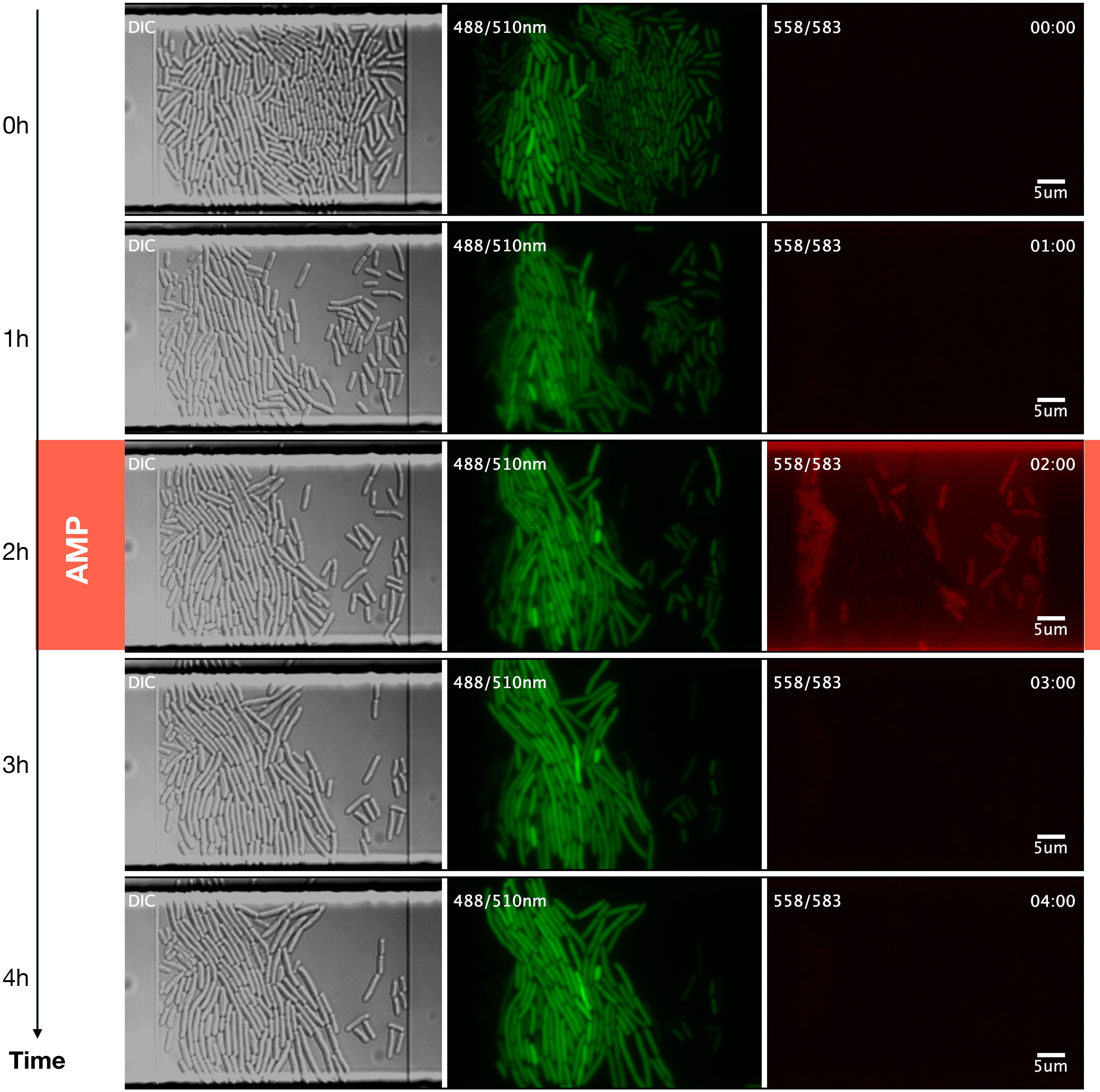
Here, we used a series of programs in \(\mu \mathrm{J}\) (https://github.com/ccg-esb-lab/uJ), which consists of an \(\mathrm{ImageJ}\) macro library (mainly) for quantifying unicellular bacterial dynamics in microfluidic devices (Schneider, Rasband, and Eliceiri 2012) (See Figure 1.1).
1.2 Preprocessing
We exported the figures obtained by the NIS-Elements software (RRID:SCR_014329) from the microfluidics experiments in TIFF (Tagged Image File Format) format. Each figure was named as follows: experimentxyc1t001, where experiment indicates the name assigned to the experiment, xy the trap number, c the fluorescence channel, and t the passage of time.
Subsequently, we compile the images, rename them and save them as images in different folders. We maintained the classification by fluorescence channels and phase contrast, and within the channel folder, it is the sub-classification by trap number.
1.3 Segmentation
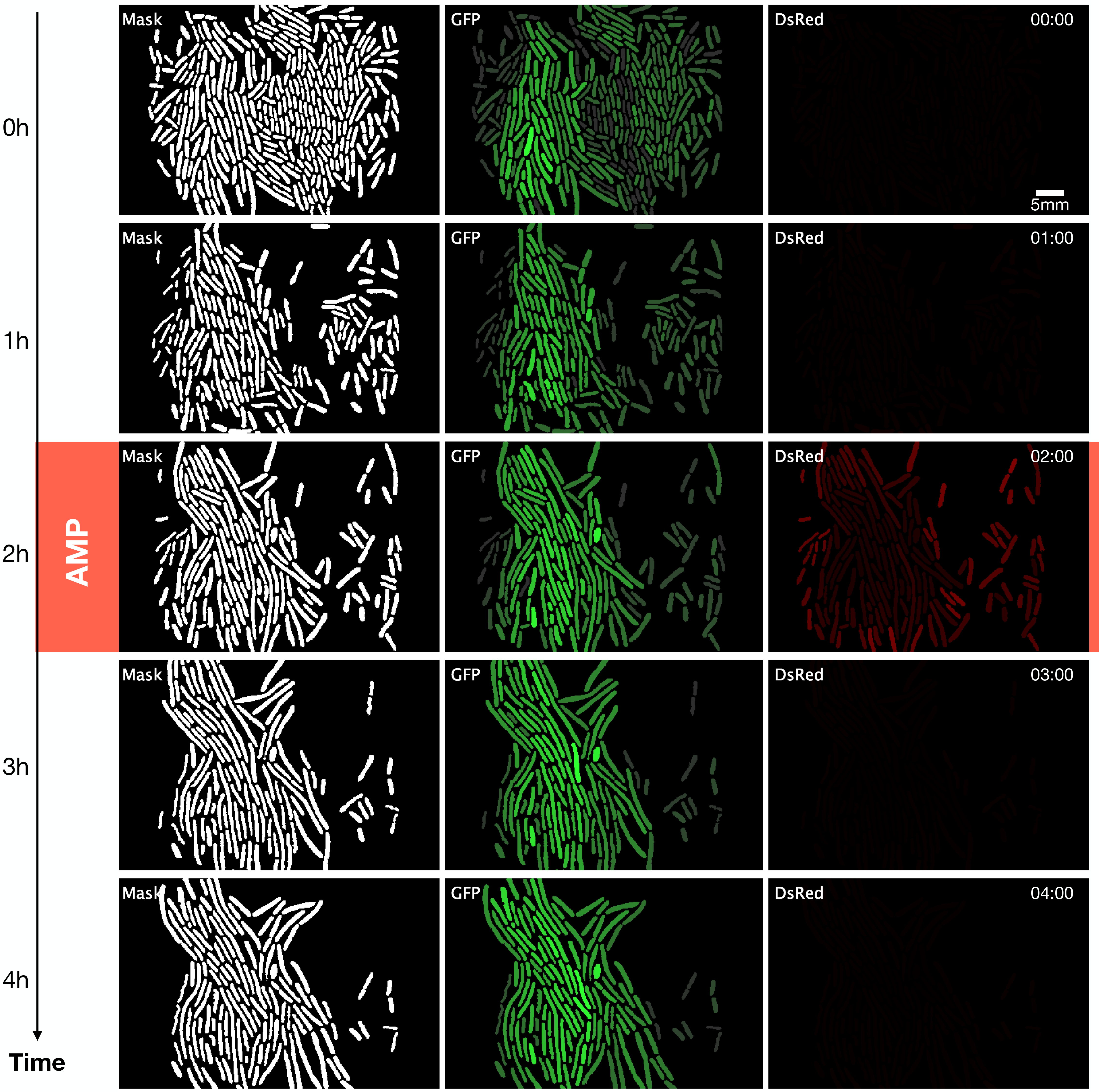
We carry out an image segmentation analysis to determine which parts of the photographs correspond to cells (See Figure 1.2). Segmentation consists of classification at the pixel level, which allows us to define the pixels that give identity to the limit of a cell, its interior, and the image’s background (everything that is not a cell). The resulting image is the segmentation mask, containing only the pixels that identify cells.
To build the segmentation mask, we used Deepcell (Van Valen et al. 2016). Deepcell is a network trained with a robust set of images that people previously classified as cells. However, the generation of the segmentation masks is not absolved of errors (see also Section 1.5). Sometimes we must correct them manually due to
mistakenly identifying two or more cells as one,
identifying two or more cells when there is only one cell, and
failing to identify a cell.
1.4 Tracking
From the image segmentation, we obtain ROI files (region of interest), which contain coordinates of the position of individual cells in each photograph (Brinkmann 2008) (See Figure 1.3). Tracking is following a region of interest in a consecutive series of images. In this case, the tracking identifies the lineages, that is, the ancestry of each cell.
We read the ROI files in Python through the shapely package, which efficiently reconstructs polygons, thus calculating the length of the cells (Van Rossum and Drake 2009; Gillies et al. 2007--). Also, in Python, using ROI files, we track cells with the k-nearest neighbors’ algorithm that uses various cell properties, such as fluorescence intensity, length, and shape of each cell, to identify cell lineages (Altman 1992).
![]()
1.5 Manual corrections
For cell-tracking manual correction, we used Napari, an open-source python-based tool designed to explore, annotate, and analyze large multidimensional images (Sofroniew et al. 2021). Our custom cell-viewer allows us to easy lineage data visualization, custom-plotting, and lineage correction. Code for our cell-viewer is available on https://github.com/ccg-esb-lab/uJ/tree/master/single-channel.
We produced high-throughput data of thousands of cells with a single-cell resolution to the end of the lineage manual reconstruction. We obtained data on the time series of fluorescent intensity, morphological properties of individual cells (e.g., elongation, duplication rate), and time-resolved population-level statistics (e.g., probability of survival to the antibiotic shock).
1.6 Data extraction
We construct a file in columnar format through image processing that contains the information necessary to analyze each experiment (i.e., chromosomal and plasmids) in its different traps (i.e., XY identifier). See Table 1.1 for a complete description of the output data. Subsequently, the table was analyzed in R for statistical computation and plotting (see Chapter 2) (R Core Team 2022).